Function extraction in IoT malware samples, a comparative study

Study about pursuing two primary objectives: implement a loosely coupled software component responsible for encapsulating a function extractor backend, execute a fair and empirical comparison of Ghidra, radare2 and angr in terms of function extraction performance.

Introduction

Over the past decade, the proliferation of Internet of Things (IoT) and embedded devices has created a new frontier for malicious actors. In these environments, established security best practices and solutions are often absent or infeasible to implement. Consequently, the scale of exploitation has surged, introducing unprecedented volumes of threats, as demonstrated by the Mirai botnet (Antonakakis et al., 2017).

The public availability of IoT malware source code has exacerbated this issue. Threat actors frequently reuse code to create custom variants, resulting in complex, overlapping relationships between malware families. While each variant introduces new capabilities that require specific countermeasures, the high degree of code reuse often leads traditional Anti-Virus (AV) solutions to misclassify samples and fail to capture the underlying code-sharing dynamics prevalent in IoT malware ecosystems.

State-of-the-art AV solutions rely on automated pipelines and models, such as clustering, rather than manual analysis for malware labelling. The efficacy of these clustering models heavily depends on the underlying similarity metric. Cozzi et al. (Cozzi et al., 2020) demonstrated that traditional clustering based on static and dynamic features is insufficient to identify meaningful similarities or isolate variations among sub-families. Conversely, code-based similarity proved effective in tracking the evolutionary timeline of specific families and identifying functions borrowed across different lineages.

Conducting function-level code similarity analysis requires accurately disassembling the binary and extracting its constituent functions. While this task is trivial for unstripped binaries, IoT malware is frequently stripped. The absence of a symbol table (.symtab) necessitates the use of complex heuristics to identify function boundaries.

Several modern disassemblers and binary analysis frameworks implement heuristic-based function boundary identification and code extraction. However, there remains a significant gap in the literature regarding the accuracy, performance, and scalability of these tools for ARM and MIPS architectures, which are typical of IoT malware.

This study addresses this gap by pursuing two primary objectives. First, this work proposes a novel, loosely coupled software component that encapsulates the function extraction backend. By defining a standardised interface for function extraction, this component enables interchangeable backends, significantly streamlining integration into broader malware clustering pipelines. Second, it presents an empirical evaluation of three prominent tools: Ghidra, radare2, and angr, comparing their performance and scalability in identifying and extracting function boundaries from stripped IoT binaries, using the software component achieved in the first objective.

The remainder of this document is structured as follows: Section  2 elaborates on why this study matters, highlighting the critical need for accurate function extraction in automated malware analysis pipelines. Section  3 provides the necessary technical background on stripped binaries, boundary identification heuristics, and the specific disassemblers evaluated in this work. Section  4 details the proposed approach, outlining the methodology for the empirical comparison and the architectural design of the loosely coupled extraction component. Section  5 presents the empirical findings of the study, regarding the performance of the examined disassemblers. Section  6 covers possibilites, where the study and its deliverables can be improved in the future.

Why this study matters

Traditional automated malware analysis pipelines heavily rely on clustering algorithms driven by high-level static metadata and dynamic behavioral features (Dumitras & Neamtiu, 2011; Jang et al., 2011; Karim et al., 2005; Lindorfer et al., 2012). However, these traditional metrics frequently fail to capture the complex, overlapping code-sharing relationships inherent in modern IoT malware ecosystems (Cozzi et al., 2020). Clustering based strictly on static and dynamic features often yields suboptimal and unreliable groupings: models may become too granular and overspecific, failing to connect minor variants of the same lineage, or they may become too coarse, mistakenly grouping functionally distinct malware families based on superficial similarities.

To overcome these limitations, state-of-the-art analysis has shifted toward function-level binary code similarity. By mathematically comparing the actual compiled functions, security systems can accurately track code reuse, evolutionary lineage, and borrowed capabilities across different threat actors, regardless of superficial obfuscation.

However, the efficacy of function-level similarity is entirely contingent upon a critical prerequisite: the accurate identification and extraction of function boundaries from the underlying stripped binary. If this foundational extraction phase is flawed, whether by missing functions, misidentifying entry points, or incorrectly splicing assembly instructions, the resulting similarity calculations will be inherently compromised, rendering the downstream clustering ineffective.

Furthermore, accuracy alone is insufficient for modern threat intelligence. Given the unprecedented volume of newly generated IoT malware variants, the boundary identification and extraction solution must also be highly performant and scalable. An extraction heuristic that achieves high accuracy but requires excessive computational overhead cannot be viably integrated into a high-throughput, automated malware triage pipeline.

This study matters because it directly addresses this operational bottleneck. By empirically evaluating the accuracy and scalability of prominent binary analysis frameworks (Ghidra¹, angr², and Radare2³), this research provides the cybersecurity community with the data-driven insights necessary to select the optimal backend for function extraction. Moreover, by proposing a standardised, loosely coupled extraction component, this work ensures that accurate, scalable function extraction can be seamlessly integrated into existing machine learning pipelines, bridging the gap between theoretical code similarity and practical, large-scale threat defence.

Background

ARM assembly

Defining and understanding Assembly language, more precisely ARM assembly, especially in the IoT environment, is essential in approaching the problem of function code extraction and boundary identification.

Assembly language is essentially a thin abstraction layer, with its own syntax, on top of the machine code layer, which is composed of instructions that are encoded in binary representations (machine code), which is what a computer understands. However, when humans would like to run an instruction, or better said, a set of instructions, called a program, on a computer, the language barrier of machine code would profoundly encumber the process of programming. Therefore, assembly was introduced to make the transaction of code at the lowest level, between a programmer and a computer. Assembly code is then assembled to machine code. Since the inception of this idea, higher demand for complex software, therefore shorter development lifecycles, created the need for higher-level programming languages than assembly, but ultimately, every advanced software is systematically reduced to architecture-specific assembly language at the processor level.

Assembly represents the binary machine code with mnemonics, abbreviations where each machine code is given a representative name. A programmer uses these names as instructions. The operands of an instruction come after the mnemonic(s).

ARM architecture is a RISC (Reduced Instruction set Computing) processor, and consequently has a simplified instuction set. ARM uses instructions that operate only on registers and uses a Load/Store memory model for memory access, which means that only Load/Store instructions can access memory.

The number of registers depends on the ARM version. The ARM Reference Manual states that there are 30 general-purpose 32-bit registers, with the exception of ARMv5-M and ARMv7-M based processors. There are special purpose registers, which are important to note, especially those that play a crucial role in function prologue and epilogue.

R13,alias the SP (Stack Pointer) register, points to the top of the stack. The stack pointer changes whenever a PUSH or POP instruction happens. The stack is an interval of memory utilized for function specific storage, which is reclaimed when the function returns. Allocation or deallocation can be achieved by modifying the SP.

R11, alias the FP (Frame Pointer) register, points to the bottom of the current stack frame. To separate functions context, stack frames are used, which is a localised memory portion within the stack that is dedicated for a specifig function. The frame usually contains the return address, previous Frame Pointer, any registers that need to be preserved and function parameters, in case they are not passed in registers.

R14, alias the LR (Link Register). In the event of a function call, the value of the memory address referencing the next instruction where the function was called from is written into the LR. This enables the program to return to the caller function after the callee function finished.

Functions in ARM can be broken up into three structural parts: a prologue, a body and an epilogue. The prologue is used to save the previous state of the program by taking advantage of the stack. It's also the responsibility of the prologue to set up the stack for the local variables of the function. The exact implementation of the prologue may differ between compilers. The body part contains the logic the function is supposed to follow. The body can also contain branching to other functions, making the calls of functions nested. Symmetrically to the prologue, the epilogue restores the state of the program as it was before the function call. This includes updating the SP register with the current value in the FP register, and restoring the saved register from the stack.

Function epilogue and prologue can differ, depending on whether the function is a leaf or a non-leaf function. A function is considered a leaf if it does not branch to another function from itself. Non-leaf functions, in addition to their own logic, branch to another function.

The Executable and Linkable Format (ELF)

To comprehend the challenges of automated binary analysis, one must first understand the structural container in which compiled code is distributed. In the context of IoT devices, which are predominantly powered by Linux-based operating systems, the Executable and Linkable Format (ELF)⁴ serves as the de facto standard for binaries, shared libraries, and core dumps.

The ELF specification defines a highly structured dichotomy, organising the binary into two distinct perspectives: the Linking View (used by the compiler and linker during creation) and the Execution View (used by the operating system's loader when launching the program).

The ELF Header

Every ELF file begins with a mandatory ELF Header. This header contains metadata that dictates how the rest of the file should be parsed. For cross-architecture IoT malware analysis, the following fields are of importance:

• e_machine: This field explicitly defines the target instruction set architecture (ISA), such as ARM, MIPS, or x86-64. Automated disassemblers rely entirely on this byte to select the correct lifting engine and instruction semantics.

• e_entry: This field provides the virtual memory address of the program's entry point---the exact location where the operating system transfers control to begin execution. While this provides the start of the first function (typically _start), the boundaries of all subsequent functions remain undefined in the header.

• e_shoff: This field contains the offset to the section headers table, in which each header holds metadata of its section.

• e_shnum: This field provides the number of entries in the sections headers table.

• e_shentsize: This field holds the size of a section header.

The e_shoff, e_shnum and e_shentsize are described because their values can be mangled with, achieving anti-analysis, without compromising the execution of a binary.

Sections

Within the Linking View, an ELF file is divided into various sections, each serving a specific semantic purpose. The most critical sections for reverse engineering include:

• .text: This section contains the actual executable machine code (the compiled assembly instructions).

• .rodata and .data: These sections hold read-only data, such as hardcoded strings, and initialised global variables. Disassemblers frequently use cross-references from the .text section to strings in the .rodata section as a heuristic to identify the beginning of error-handling or logging functions.

Segments

Unlike sections, segments are memory-oriented divisions of an ELF file, designed for the OS loader. They describe how to map the ELF file into the virtual address space of a process during execution. Segments group data by memory attributes (e.g, read-only, executable) rather than logical content.

Stripped and unstripped ELF binaries

A consequential component of the ELF format for this study is the presence or absence of debugging metadata and symbol tables. The dichotomy between an unstripped and a stripped binary fundamentally alters the complexity of reverse engineering and automated analysis.

Unstripped binaries:

When a compiler generates an ELF file by default, it produces an unstripped binary. This file contains a wealth of metadata designed to aid developers in debugging. Structurally, an unstripped ELF includes:

• .symtab (Static Symbol Table): A contiguous array of entries that maps every internal function name and global variable to its exact memory address and byte size.

• .strtab (String Table): Contains the human-readable character strings representing the names of the symbols referenced by the .symtab.

• .debug_* sections: If compiled with debug flags (e.g., -g in GCC), the ELF includes DWARF debugging data, which can map raw assembly instructions directly back to the specific lines of the original C/C++ source code.

In an unstripped binary, extracting function boundaries is a trivial $\mathcal{O}(1)$ table lookup. Disassemblers simply parse the .symtab to locate the exact start address and length of every function.

Stripped binaries:

To minimize the binary footprint for constrained IoT environments and to implement a basic layer of anti-analysis obfuscation, malware authors routinely utilise stripping prior to deployment. Stripping fundamentally alters the Linking View of the ELF file while leaving the Execution View intact.

A stripped binary can undergo a spectrum of changes, depending on how the stripping utility is configured. With the default configuration, the following structural changes are made:

• The .symtab, .strtab, and all .debug_* sections are permanently deleted.

• The Section Header Table, which acts as the directory for these sections, is modified or completely removed.

If the malware is dynamically linked (relying on external libraries like libc), the .dynsym (Dynamic Symbol Table) must remain intact for the operating system loader to resolve external calls (e.g., printf or socket). However, .dynsym only exposes imported and exported symbols; it does not contain the internal functions written by the malware author.

Because the operating system relies exclusively on the Program Headers (the Execution View) to map the .text instructions into memory, stripping does not affect the malware's execution. However, when analysis frameworks like ghidra, radare2, and angr ingest a stripped ELF binary, they are presented with a continuous, unstructured block of executable bytes. The absence of the .symtab forces these frameworks to abandon deterministic lookups and rely entirely on heuristics to reconstruct the lost function boundaries.

Metrics

The metrics computed and collected during a measurement are the basis of every conclusion and result of a study. A simple accuracy metric often fails to capture the reasons and the real image of the performance of a given tool, since it hides the metrics of false negatives and false positives.

Precision and recall

Precision

is the ratio of true positives and all retrieved positives. It could be explained as the fraction of correctly identified functions among all the identified functions.

Recall

is the ratio of true positives and all actual positives. Similarly, this could be used to retrieve the information of the fraction of correctly identified functions among all the identified functions.

Edit distance

Edit distance (Ristad & Yianilos, 2002) is a string metric where the way of quantifying how dissimilar two strings are to one another is by counting the minimum number of operations required to transform one string to the other. Different applications of edit distance define different sets of operations. For example, the Levenshtein distance defines the insertion, deletion or substitution of a character in a string.

In terms of function boundary identification, string comparison is not relevant. However, one application of edit distance, the set edit distance, computes a distance between the input set x and the input set y, given the element-wise edit distance delta function. In more detail, the function finds an assignement $M=(i,j), i\in \{1,..,len(x)\},j\in \{1,..,len(y)\}$ where the following loss in minimalized:

$\sum_{(i,j) \in M }^{}\delta(x_i,y_j) + \sum_{i \notin M }^{}\delta(x_i,-) + \sum_{j \notin M }^{}\delta(-,y_j)$

This problem can be solved with the Hungarian method (Kuhn, 1955).

A delta function is required to define the element-wise loss, where the combinations to be considered are:

• For a given $x_i$ where there is no $y_j$. This can be interpreted as an insertion of an element from the set y.

• For a given $y_j$ there is no $x_i$. This can be interpreted as a deletion of an element from the set y.

• For a given $x_i,y_j$, where both elements are present.

Approach

In this section, we describe our approach, which was designed to reach the objectives established by us. First, we define the model for the measurement method, ensuring that it is fair towards the examined tools, and that is sound with the performance of the tools. Second, we cover the software component responsible for the encapsulation and the implementation of the measurement model. A brief overview of our approach can be seen in Figure 1.

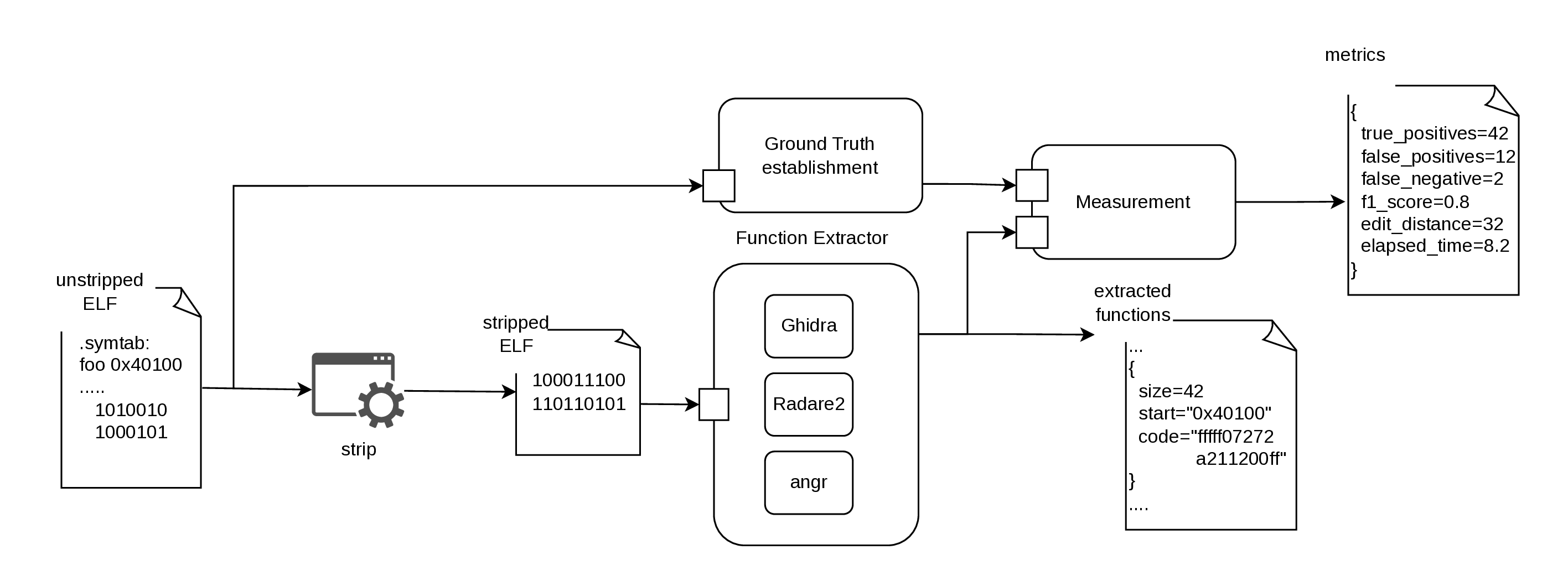Figure 1: Overview of the approach to the measurement.

Measurement model

The following sections elaborate our model of measuring function boundary identification accuracy on different abstracion levels, and the reasons behind the decisions related to different aspects of the approach. Additionally, we describe the limitations of the approach.

Ground truth establishment

For the measurement to be at most accurate, a standard and fair comparison should be stated. The main methodology to measure the performance of a disassembler in function boundary identification, is similar to any supervised assertion or test, where we compare the output of the examined tool or function, to a ground truth. A ground truth is defined as a de facto base of comparison, which we firmly belive to be true. In our context, this can be an unstripped version of the target binary, in which function extraction is trivial, and the true function boundaries can be established by reading the entries from the .symtab section. Furthermore, it is crucial to the fairness of the comparison that the establishment of the ground truth is independent from all of the tools under examination. This is simply required, so the results won't be biased in favor of any of the tools. Our approach follows this idea.

Comparison targets

Comparing ground truth and extracted functions begs the question of in what way we can measure the similarity of given functions. The scope of the study suggests that the goal is to measure the performance of a disassembler in its ability to identify function boundaries, therefore the boundaries should be the ones to be compared. One would suggest to compare the functions on a binary code level, however that would be excessive in this case, since the ground truth and the target binary are required to be the same on a binary level, and the extracted binary code only depends on the extracted boundary of a given function. A common way to define function boundaries is, the start address and the size of the function. We decided to proceed with this definition. The ground truth function boundaries are read from the unstripped versions of the target binary, and the measured functions are extracted with the examined tools, from the stripped versions of the binary.

Model

To solve the similarity calculation between function boundary sets, we came up with the following model. We have a set of function boundaries from the ground truth and another set from the target binary. This can be perceived as a bipartite graph, where one set of vertices are the truth boundaries, and the other set is the extracted boundaries. From each vertex in the truth set, an edge connects to every vertex in the extracted set, and vice versa. On each edge, a delta value should be noted, which would indicate the difference, or more commonly, the cost between the two boundaries. For this model to be accurate with our objectives, a virtual vertex should be defined for each vertex in both sets, where the delta value is interpreted as if there is no matching boundary in the opposite set. The described model is visualized in Figure 2. In this problem, we need to find a matching of vertices, along the edges, where the sum of the delta values are minimalized. This minimization is necessary because the delta value effectively acts as a distance or error cost---where a lower value represents a tighter alignment between boundaries, and a delta of zero indicates a perfect match. Matching a real vertex to a virtual vertex imposes a fixed penalty cost representing a false positive (hallucinated boundary) or a false negative (missed boundary). By minimizing the total sum of these edge weights, we frame our evaluation as a Minimum Weight Bipartite Matching problem. This mathematically guarantees that we find the globally optimal alignment, one that naturally balances the trade-off between penalizing slightly shifted functions and punishing completely missed ones, thereby providing a rigorous reflection of the disassembler's true accuracy.

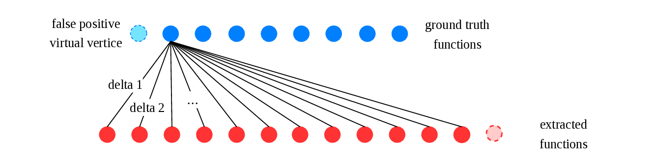Figure 2: Functions represented as a bipartite graph with virtual vertices.

The presented model and the Minimum Weight Bipartite Matching problem are solved by the set edit distance. The set edit distance depends on a delta function, in the same relation as described above in the bipartite graph model. The output edit distance will be used as the number one indicator of a disassembler's performance on a given binary sample.

Delta function:

A delta function must implement the three fundamental combinations of inputs, as it was established above. For the function itself, multiple candidates were considered. At first, a simple Euclidean distance was studied, as the distance between two function boundaries on the 2D plane, where the coordinates are the start and the size of a boundary. However, we realised that there is a fundamental flaw in this interpretation of a boundary. That is, in a standard Euclidean distance, the start address and the size are treated equally, symmetrically and independently, whereas binary functions inherently reside in a 1D memory space, where these two variables are strictly coupled. Consider the following example: assume a target binary where the ground truth function boundary is defined by its starting address and size as a tuple $B = (start, size)$. Let the ground truth boundary be $B_{GT} = (1000, 50)$, meaning the function occupies the one-dimensional memory interval $[1000, 1050)$.

To evaluate the mathematical penalty of incorrect extractions, we examine two distinct errors a disassembler could make:

Scenario 1: Address shift

The disassembler incorrectly calculates the start address but gets the size right, outputting $B_1 = (1050, 50)$. This boundary occupies the memory interval $[1050, 1100)$. The real-world overlap with the ground truth is exactly $0$ bytes. However, calculating the Euclidean distance $d_E$ yields:

$d_E(B_{GT}, B_1) = \sqrt{(1000 - 1050)^2 + (50 - 50)^2} = \sqrt{(-50)^2 + 0} = 50$

Scenario 2: Size shift

The disassembler correctly identifies the start address but overestimates the size, outputting $B_2 = (1000, 100)$. This boundary occupies the memory interval $[1000, 1100)$. Unlike the first scenario, this extraction successfully captures all $50$ bytes of the original function, albeit with additional trailing data. Calculating the Euclidean distance yields:

$d_E(B_{GT}, B_2) = \sqrt{(1000 - 1000)^2 + (50 - 100)^2} = \sqrt{0 + (-50)^2} = 50$

According to the Euclidean model, $d_E(B_{GT}, B_1) = d_E(B_{GT}, B_2) = 50$. The metric assigns the exact same penalty to an extraction that completely misses the target function as it does to an extraction that successfully captures $100\%$ of the target's original bytes. We know that those mistakes shouldn't be equal, since the first mistake resulted in 0 bytes overlapping, whereas the other was 50 bytes correct. The incorrectness of this model is visualized in Figure 3. Furthermore, an unweighted Euclidean distance struggles to elegantly represent the fixed penalty required for mapping to virtual vertices (representing false positives and false negatives) Consequently, the Euclidean model was discarded.

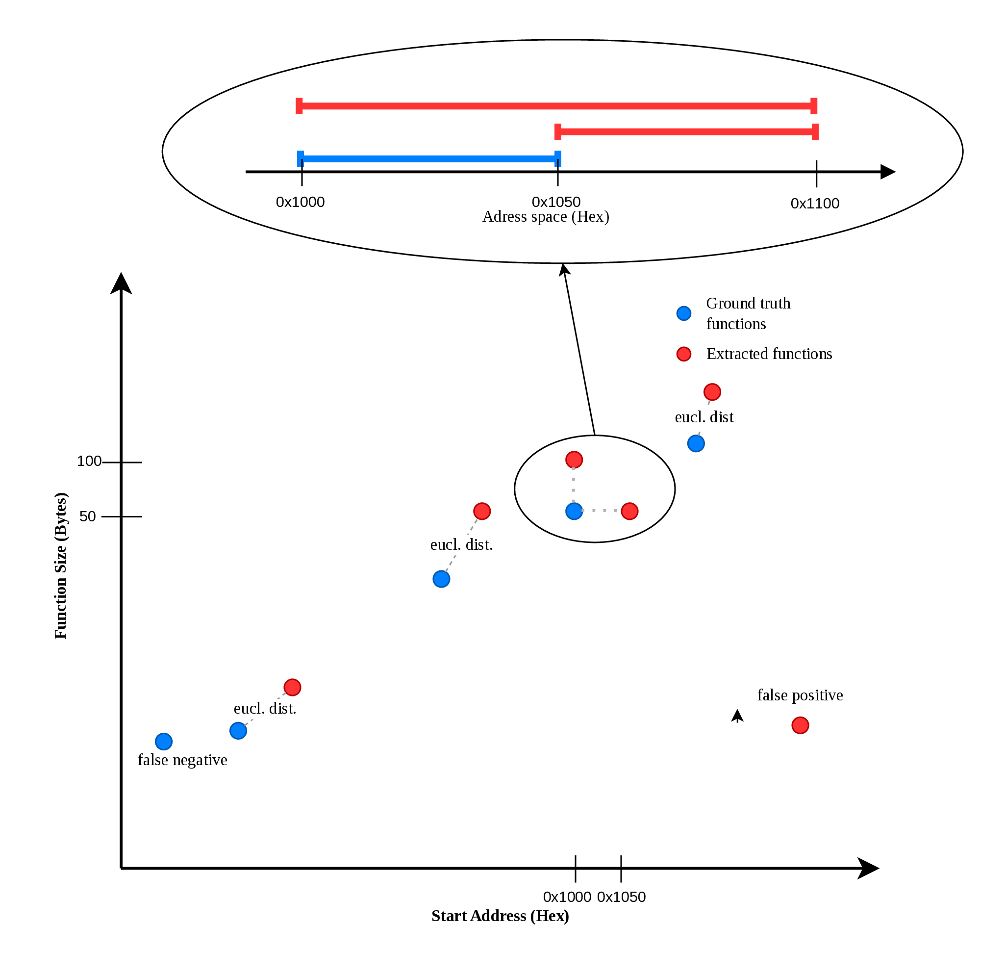Figure 3: Example function boundary comparison with Euclidean distance on a 2D plane.

On the contrary, to quantify this memory overlapping mathematically, we adopted the Intersection over Union (IoU), also known as the Jaccard index, as the primary metric. IoU calculates the ratio of the intersecting bytes (the memory addresses that both the ground truth and the extracted boundaries agrees upon) to the union of bytes (the addresses claimed by either of the boundaries). IoU is visualised in a simple example in Figure 4. Unlike the Euclidean distance, IoU treats the start address and the size bounded, in a 1D memory space. Furthermore, IoU elegantly normalizes similarity to a strict bound between 0 (completely disjoint) and 1 (a perfect match). Under this model, a perfect alignment incurs a cost of 0, partial overlaps incur a fractional cost, and mappings to virtual vertices, representing missed or hallucinated boundaries, incur the maximum penalty of 1. Because set edit distance requires a delta function with cost and not similarities, the final delta costs will be $1-IoU$. This provides a mathematically robust, bounded metric that perfectly satisfies the constraints of the Minimum Weight Bipartite Matching problem. It is fundamental for the correctness of IoU, and that our model is aligned with how functions are in binaries, we assume that functions are continuous memory chunks.

Figure 4: Example functions and their intersection and union.

Additional metrics

Additionally, besides the edit distance, we decided to measure the number of true positives, false positives and false negatives of function boundaries, as indicators of performance, which are more intuitive to understand for the humand mind. We also decided to account for, and measure the elapsed time of function extraction, since it's valuable information in judging the scalability of a given disassembler.

Constraints

During the measurement, on number of unforeseen variables, several constraints had to be set, for the sake of achieving the established objectives in the time window of the study, while remaining in the scope of the project. The dataset comprises real-world malware samples, which frequently employ adversarial anti-analysis techniques or suffer from structural corruption. These constraints are based on the observations made during the measurement.

Firstly, out of the 19866 samples, only 15385 were successfully stripped by the cross-platform binary parser called lief.

Secondly, structural pre-validations had to be enforced on binaries. It was observed that certain intentionally mangled binaries advertise an impossible number of ELF sections, triggering runaway memory allocation in Ghidra. This phenomenon, effectively acting as an anti-analysis memory bomb, led to Out-Of-Memory (OOM) host kernel terminations. Related to this, several samples contained impossible addresses in their ELF header. To mitigate these, pre-flight header validation method was introduced to preemptively reject malformed or zero-byte artifacts generated during the binary stripping phase, therefore these samples were not included in the measurement.

Additionally, the measurement extended only for statically linked samples, but we found that dynamically linked samples only accounted for 2.6% in the whole dataset, as it is rare for IoT malware to be dynamically linked.

Function extractor

To study the performance of disassemblers on a large scale, our first goal was to implement a software component responsible for encapsulating various disassembler backends. During the development, the main objective was to create an interface that is loosely coupled and independent of the exact disassembler in use. We followed this, in case the component is chosen as the main function extractor in a malware analysis pipeline later on, with the selected disassembler backend. The implementation was preceded by modelling the problem of measurement, and the modelling of the software itself.

Model

The implementation of the software component was based on a model, which can be seen in Figure 5. The model declares an IDisassembler interface, which encapsulates and hides the exact Disassembler implementation. Each Disassembler must implement the IDisassembler interface this way, in case a new Disassembler is introduced, the present code doesn't need to be modified. Furthermore, in Figure 6, the types, which the model uses are presented.

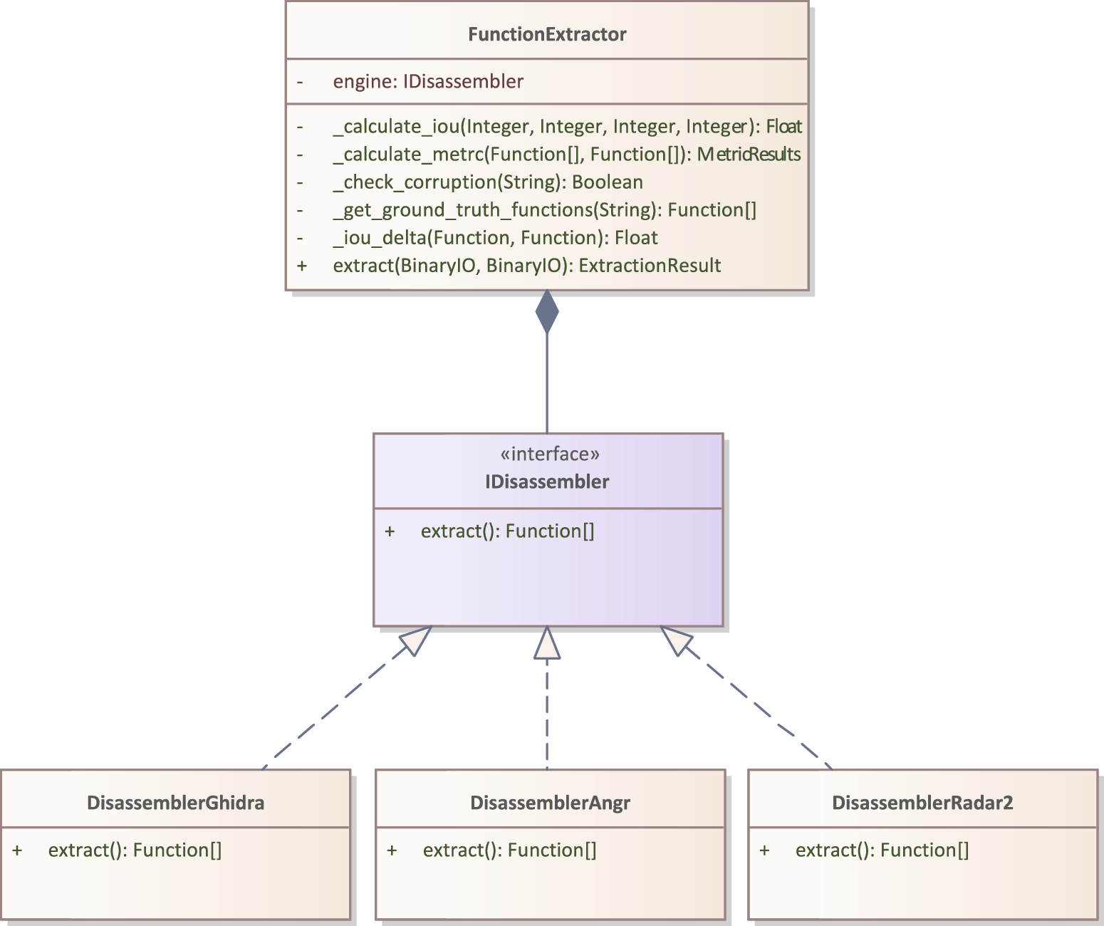Figure 5: UML Class Diagram for the Disassembler interface

Figure 5: Types used in the model

The FunctionExtractor class follows Dependency Injection as a design pattern, as its Disassembler dependency is provided from the outside. The methods present in the class, was not present during modelling, rather the model was extended as non-functional requirements were introduced during the implementation.

FastAPI

For the implementation, a framework and an environment had to be chosen. We chose FastAPI, because it's a modern and high-performance web framework for building APIs with Python. We could have used a web framework made in Go, considering that disassembly of multiple samples can be completely done in parallel, utilising the simplicity of writing concurrent code in Go, however we decided to continue with Python for the measurement. The reasons are as follows; Python is good for prototyping and experimenting, and the learning curve is acceptable, while still offering good performance. With FastAPI, internal logic, for example the function extraction, can be exposed via a REST API.

What the model misses to elaborate on is how FastAPI exposes the public extract function in FunctionExtractor. With FastAPI, a POST endpoint is exposed on the /api/{disassembler_name}/extract endpoint. This way, a web server is listening for HTTP POST requests on this endpoint. The endpoint follows the Factory design pattern as it constructs different FunctionExtractor engines, based on the disassemble_name parameter in the request. The documentation of the endpoint:

POST /api/{disassembler_name}/extract

Parameters

Name	Located in	Type	Description
disassembler_name	path	string	The unique identifier of the disassembler. Required.
target	multipart/form-data	file	The target binary, from which the functions are to be extracted. Required.
ground_truth	multipart/form-data	file	The ground truth binary, from which function extraction is trivial and the results can be used as truth to compare the extracted functions from the target. Optional.

Responses

Status Code	Description
200 OK	Successfully extracted the functions.
415 Unsupported Media Type	Either the target or the ground truth binary can’t be used during the measurement, for various reasons.
422 Validation Error	Invalid parameter format.

Example Response (200 OK)

            {
              "functions": [
                {
                  "boundary": {
                    "start": "string",
                    "size": 0
                  },
                  "code": "string"
                }
              ],
              "metrics": {
                "true_positives": 0,
                "false_positives": 0,
                "false_negatives": 0,
                "recall": 0,
                "precision": 0,
                "f1_score": 0,
                "setedit_cost": 0
              },
              "elapsed_time": 0
            } 

Disassemblers

The study measures three disassemblers, per se the objective established. Each disassembler is coupled to its own Adapter class via its own APIs. For example, Ghidra is used inside the DisassemblerGhidra Adapter class. It is at most important, for the sake of fairness and reproductability, that we elaborate on, how these disassemblers were called and configured during our measurements. It can be said universally for all three of the disassemblers that extracted functions, which are less than 5 bytes, are discarded to filter out PLT stubs and else. Additionally, functions are percieved and extracted as continuous chunks of memory, disregarding that certain optimalization techniques may split functions and place them in a non-continuous way.

Ghidra

The Ghidra disassembler engine utilises the pyghidra library to connect to the installed Ghdira instance.

angr

angr is used with its angr Python package. Examined samples are loaded with auto_load_libs=False to prevent angr trying to resolve and load dynamic libraries. To construct the function boundaries, a fast static control flow graph analysis (CFGFast) is executed rather than a full symbolic trace. CFGFast is called with the following parameters: normalize=False, function_prologues=True, force_smart_scan=False, resolve_indirect_jumps=True. Force smart scan was disabled because we observed that it resulted in an unreasonable amount of false positives.

Radare2

The final evaluation module utilises r2pipe to establish an inter-process communication interface with the Radare2 command-line disassembler. Upon initialising the target sample, the pipeline issues the exhaustive aaaa analysis macro. Function definitions are retrieved via the localised JSON function list command aflj.

Deployment

With the measurement and extractor component, we provide a Docker container file to ease the integration of the component, into existing pipelines and infrastructure. This way, the component can be used as a microservice, independent and decoupled to previously implemented components. The container includes all the dependencies of the service, making it portable and independent from the host system. This effort from us, also serves the ojective to enable others to reproduce our findings.

Results

The measurements were concluded on 15385 real-world malware samples, consisting of samples made for the ARM and the MIPS architecture. In the following sections, we describe our results. Additionally, we share the results in Table 1 and Table 2, which show the results as median values and Interquartile range (IQR) values, on samples for the ARM and MIPS architecture, respectively.

Execution time

Execution times across the three disassemblers on the samples built for ARM, exhibited varied distributions, as illustrated in Figure 7. It is important to note that the diagram's y-axis on Figure 7 and Figure 8 is in logarithmic scale. Ghidra and Radare2 demonstrated tightly bounded execution times on ARM, with median processing times of 8.57 and 1.86 seconds, respectively. Conversely, angr demonstrated a statistically significant variance. While its optimal baseline performance matched the other frameworks, its upper quartile extended heavily into the upper threshold, yielding a median execution time of 29.56 seconds. Based on Figure 8 it can be said that results on MIPS differs on all three disassemblers compared to ARM in aspect of execution time. The median execution time decreased to 5.32 on Ghidra, 4.85 on angr and to 0.53 on Radare2. This shows, that Ghidra and Radare2 offers a robust and predictable execution time independently from the architecture, while angr execution time depends highly on the underlying architecture.

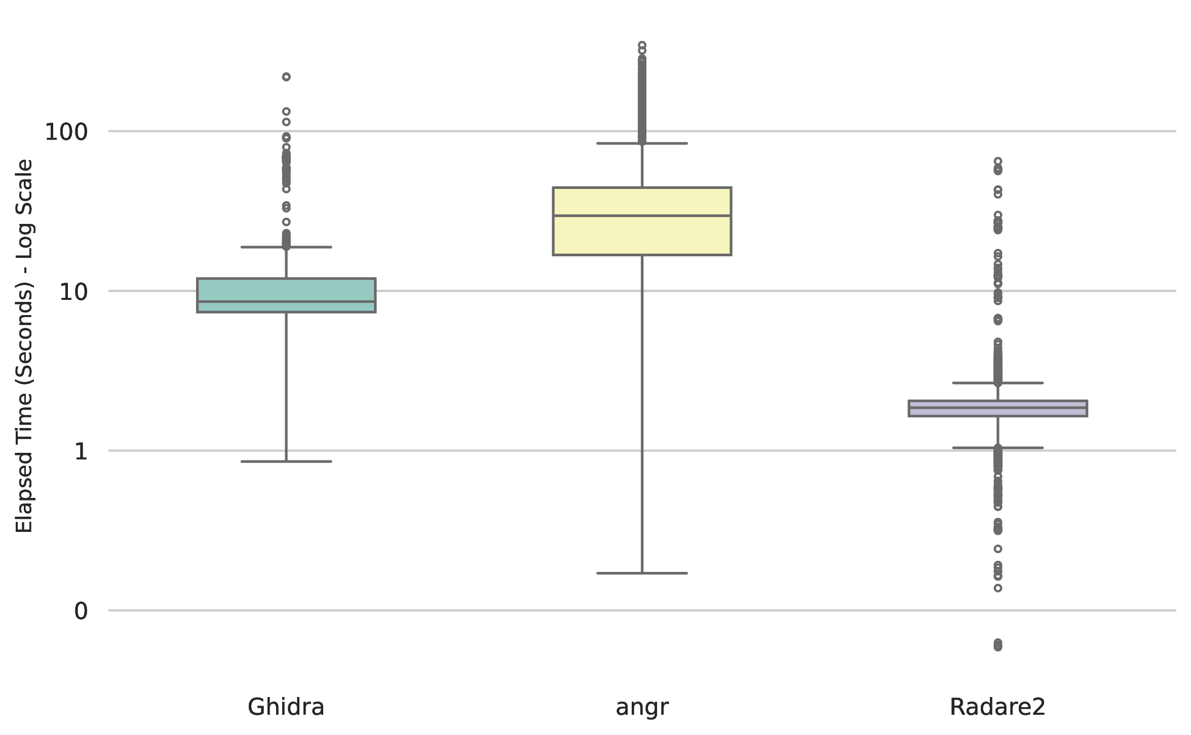Figure 7: Elapsed time (seconds) of execution wiht a logarithmic scale, ARM.

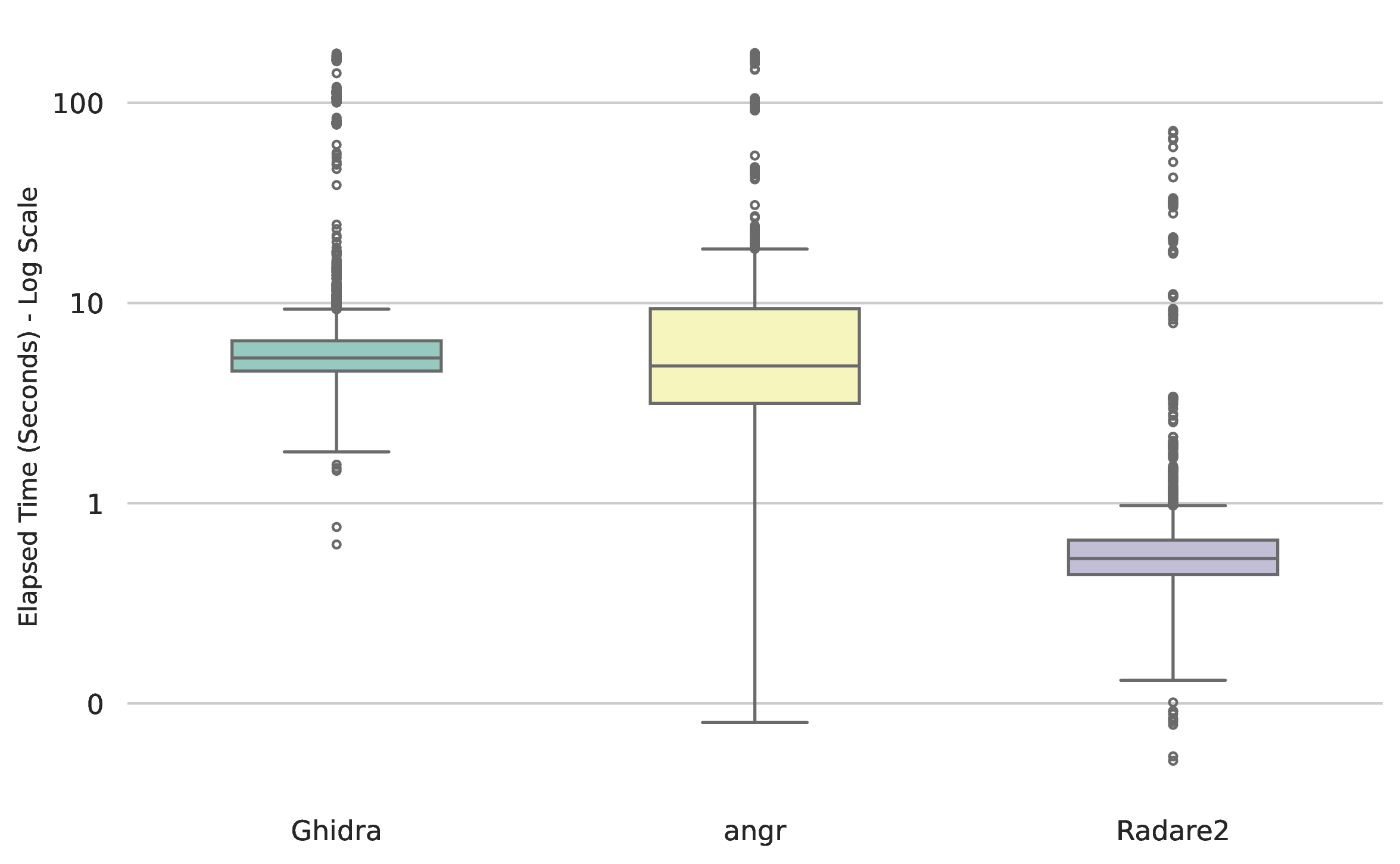Figure 8: Elapsed time (seconds) of execution wiht a logarithmic scale, MIPS.

Boundary identification

Figure 9 details the accuracy of each framework in identifying the presence of function boundaries, in samples for ARM. Ghidra achieved the highest overall detection reliability, yielding a median F1-score of 0.91, with its interquartile range heavily concentrated above 0.85. Radare2 demonstrated consistent but lower overall accuracy, characterised by a median F1-score of 0.81. angr produced the highest variance in detection capability, with an interquartile range spanning from 0.65 to 0.70, demonstrating that its structural recovery is highly binary-dependent. On MIPS, Ghidra maintains, even increases, its superiority over angr and Radare2 with a median F1 score of 0.97, as the hiearchy can be seen on Figure 10. angr completely loses its robustness, greatly fluctuating uniformly between 0 and 1 F1 score. Its 0.95 IQR value proves this behaviour. Radare2 performance also decreases fundamentally on MIPS, with a median F1 score of 0.31. To conclude, Ghidra proves to be the only robust function extractor in a cross-architecture environment, while the other disassemblers suffer greatly on architectures like MIPS.

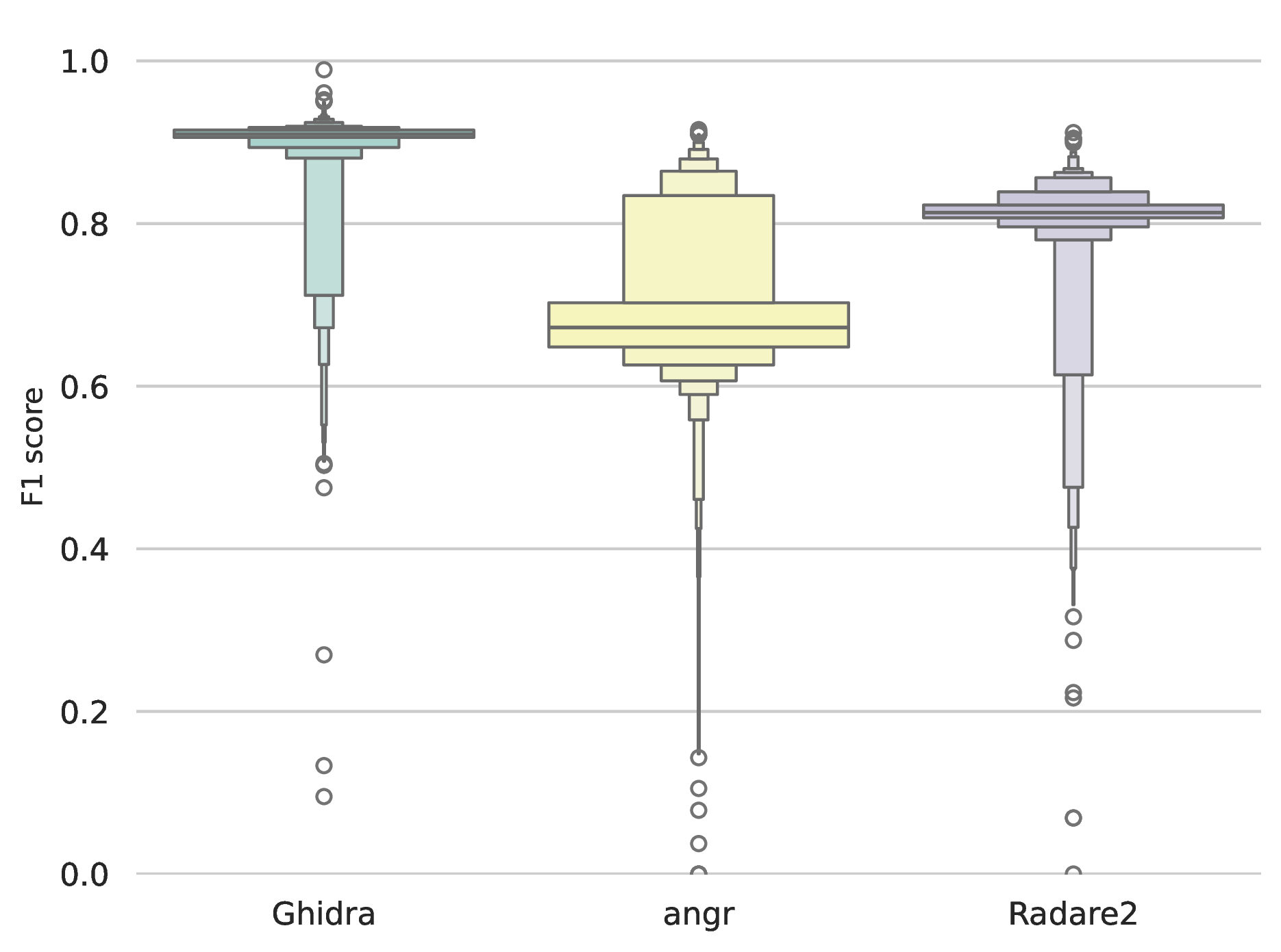Figure 9: F1 scores, ARM

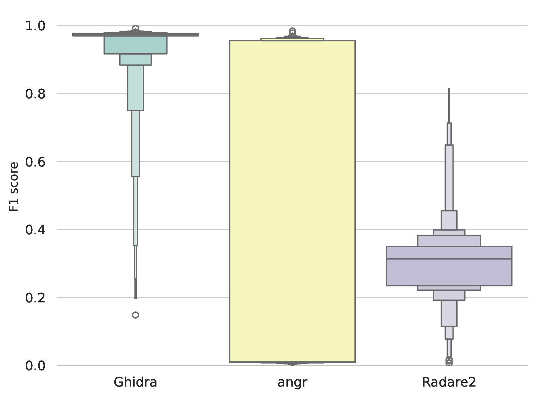Figure 10: F1 scores, ARM

Error distribution

The proportional breakdown of extraction classifications (Figure 11 and Figure 12) contextualizes the F1-scores. All of the studied disassemblers' primary error mode was False Negatives, indicating a tendency to miss functions. Radare2 exhibited a higher proportion of False Negatives. On ARM, angr's error distribution was heavily skewed toward False Positives, indicating frequent hallucinations of boundaries where none existed in the ground truth. An apparent paradox was observed in the MIPS dataset regarding angr's performance: while the aggregate error distribution chart (Figure 12) indicates a substantial proportion of True Positives, the median F1-score for angr dropped effectively to zero. This discrepancy highlights that angr achieves almost zero F1 score per binary in general, however on exceptional binaries it correctly identifies functions. Our hypothesis is that these binaries may have a higher quantity of functions, therefore they contribute much more TP to the aggregated pool, which is used in Figure 12, than the binaries where angr failes catastrophically. Additionally, it can be observed that Radare2 exhibits a lower overall proportion of True Positives compared to angr in the MIPS samples. However, the median F1 score of Radare2 on MIPS samples says otherwise. We belive that the reasons behind this inconsistency are the following. Radare2 consistently extracted a portion of functions per binary, securing a greater median F1 score, but yielded a lower absolute volume of True Positives globally, while angr's failed on the majority of samples (driving its median F1 to 0.0), but successfully extracted massive quantities of functions from a minority of outliers, thereby dominating the aggregate visual metric despite its severe lack of reliability.

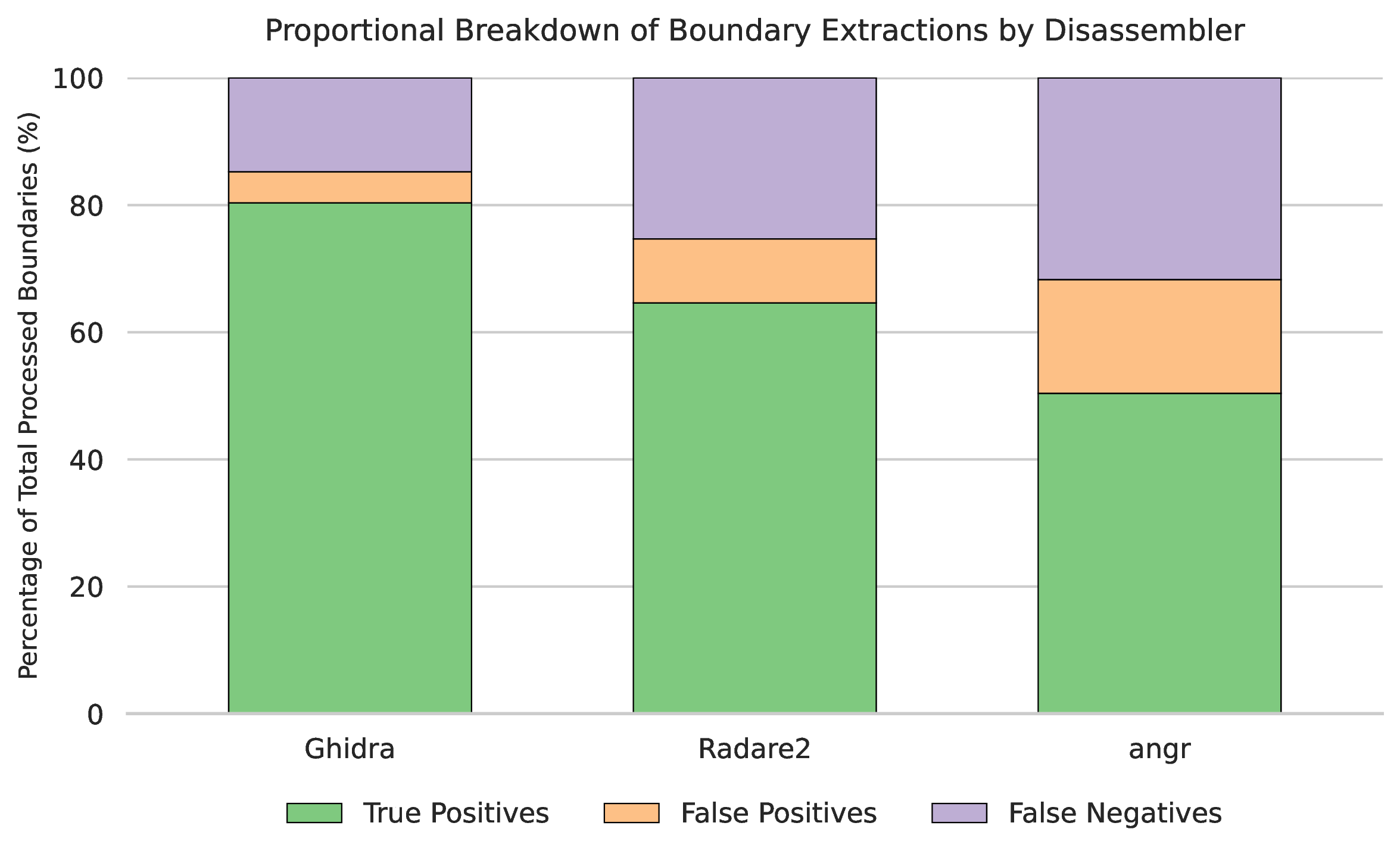Figure 9: Error (FN, FP) distribution compared to correct identifications (TP), ARM

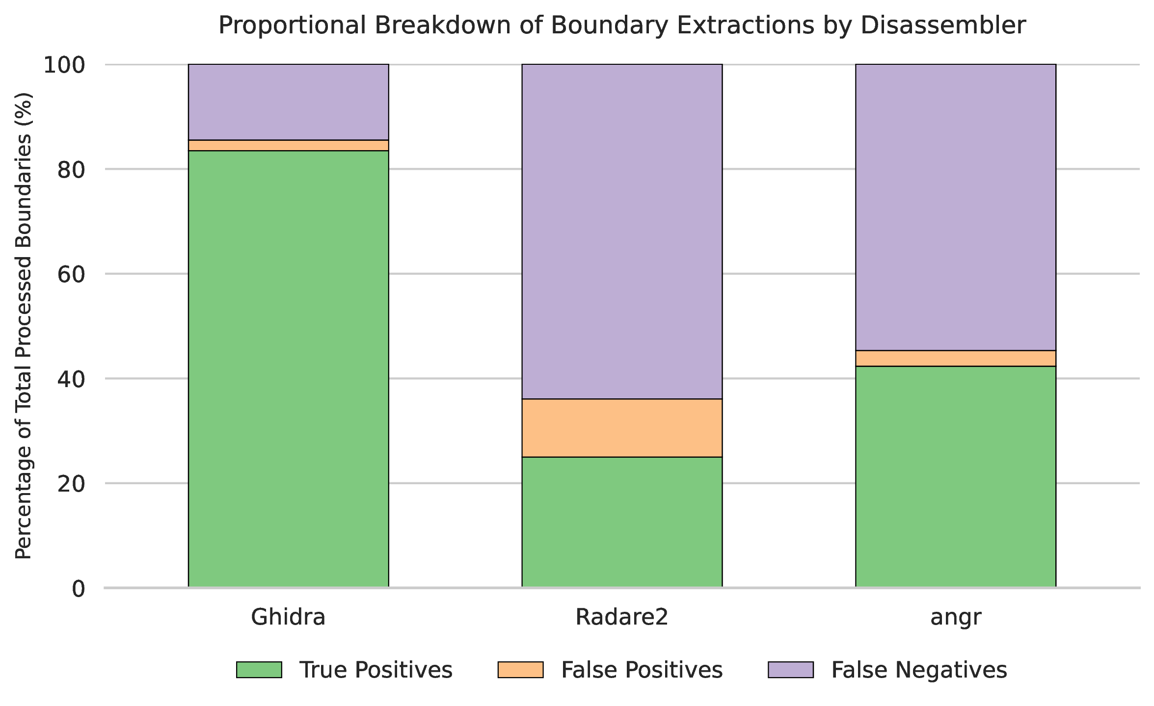Figure 9: Error (FN, FP) distribution compared to correct identifications (TP), MIPS

Boundary precision

Beyond binary detection, the exactness of the recovered boundaries was measured using the normalised Set Edit Distance. Lower values represent closer memory alignment with the ground truth. Figure 13 helps to visualize ours observations on ARM, which are the following. Ghidra achieved the highest precision, with a low variance and a median of 0.13. Radare2 produced a wider distribution peaking at 0.2, indicating frequent, minor miscalculations in function sizes. angr yielded the highest median distance of 0.26, further corroborating that while its CFG recovery may find a function, the exact start addresses and contiguous byte sizes frequently diverge from the ground truth. Figure 14 provides insights to the previously observed stark differences in the underlying behaviours of disassemblers on samples from different architectures. Ghidra demonstrated superior precision with a near zero median distance, indicating near perfect function extraction. In contrast, angr exhibited a severe bimodal distribution, with a high mass of probability concentrated around the maximum distance, which corroborates to the previously observed collapse of the F1 score. The other concentration of probality in angr's results, is around zero, proving that, indeed, there were samples in the MIPS dataset from which angr successfully extracted the functions. Radare2 displayed a different error profile. While it successfully evaded the maximum normalised distance (1.0), its error distribution is heavily concentrated between 0.6 and 0.85, with a median distance of 0.59.

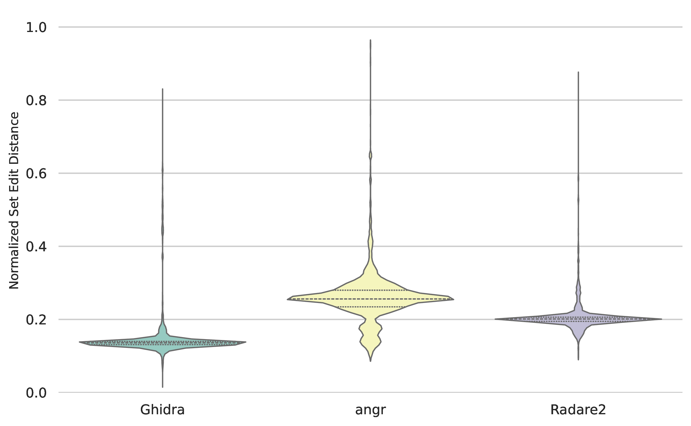Figure 13: Normalised set edit distance probability densitiy, ARM

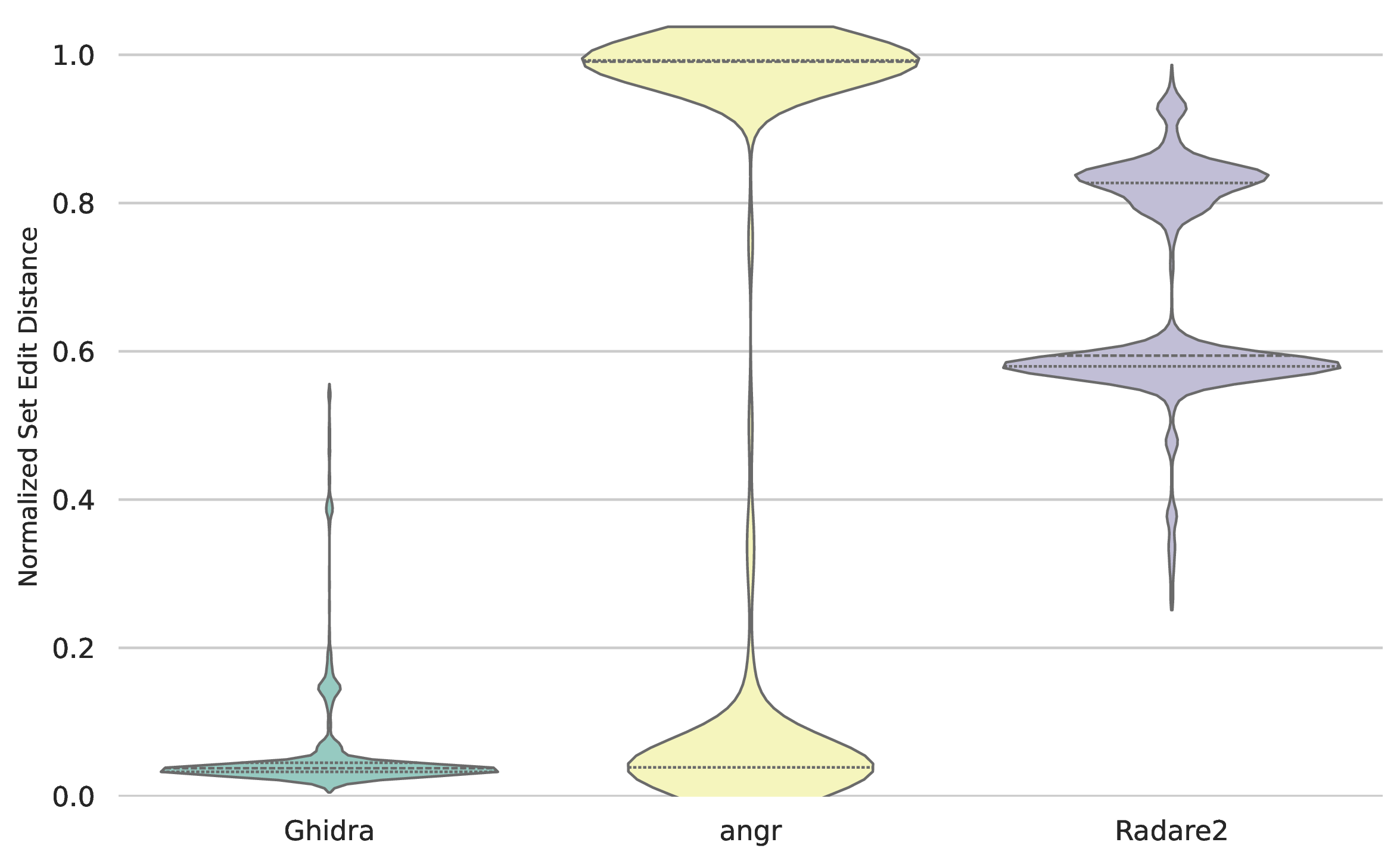Figure 13: Normalised set edit distance probability densitiy, MIPS

Future work

The measurement results provided us with the foundational knowledge to make profound decisions in the future about which tool has the best performance, depending on what we value most. Additionally, the software component was designed in a way that enables us to use it as a pipeline component later on. However, we identified two major milestones and objectives to be done in the future. First is the separation of functions defined by the user, and the library functions statically linked to the binary. Second is the scalable deployment of the software component to the pipeline.

Antonakakis, M., April, T., Bailey, M., Bernhard, M., Bursztein, E., Cochran, J., Durumeric, Z., Halderman, J. A., Invernizzi, L., Kallitsis, M., & others. (2017). Understanding the mirai botnet. 26th USENIX Security Symposium (USENIX Security 17), 1093–1110.

Cozzi, E., Vervier, P.-A., Dell’Amico, M., Shen, Y., Bilge, L., & Balzarotti, D. (2020). The tangled genealogy of IoT malware. Proceedings of the 36th Annual Computer Security Applications Conference, 1–16.

Dumitras, T., & Neamtiu, I. (2011). Experimental challenges in cyber security: a story of provenance and lineage for malware. 4th Workshop on Cyber Security Experimentation and Test (CSET 11).

Jang, J., Brumley, D., & Venkataraman, S. (2011). Bitshred: feature hashing malware for scalable triage and semantic analysis. Proceedings of the 18th ACM Conference on Computer and Communications Security, 309–320.

Karim, M. E., Walenstein, A., Lakhotia, A., & Parida, L. (2005). Malware phylogeny generation using permutations of code. Journal in Computer Virology, 1(1), 13–23.

Kuhn, H. W. (1955). The Hungarian method for the assignment problem. Naval Research Logistics Quarterly, 2(1–2), 83–97.

Lindorfer, M., Di Federico, A., Maggi, F., Comparetti, P. M., & Zanero, S. (2012). Lines of malicious code: Insights into the malicious software industry. Proceedings of the 28th Annual Computer Security Applications Conference, 349–358.

Ristad, E. S., & Yianilos, P. N. (2002). Learning string-edit distance. IEEE Transactions on Pattern Analysis and Machine Intelligence, 20(5), 522–532.

Footnotes

1. https://github.com/NationalSecurityAgency/ghidra - 2026. 05. 21. ↩

2. https://angr.io/- 2026. 05. 21. ↩

3. https://rada.re/n/radare2.html - 2026. 05. 21. ↩

4. https://www.man7.org/linux/man-pages/man5/elf.5.html - 2026. 05. 21. ↩